Motion Graphs
Motion Graphs Revision
Motion Graphs
There are two types of motion graphs: displacement-time graphs and velocity-time graphs.
Displacement-time graphs display the distance from an origin point over a period of time.
Velocity-time graphs display the velocity of a particle over a period of time.
Make sure you are happy with the following topics before continuing.
Displacement-Time Graphs
Below is an example of a Displacement-Time graph.

Some key properties about these graphs:
- The gradient represents the velocity. A steeper line indicates a greater velocity.
- When the line is horizontal, the object is not moving, (i.e. its velocity is 0).
Note:
Be wary of confusing displacement and distance – displacement is a vector quantity involving distance and a direction, distance is purely the distance from the origin, without a specified direction.


A Level Maths Predicted Papers 2024
The MME A level maths predicted papers are an excellent way to practise, using authentic exam style questions that are unique to our papers. Our examiners have studied A level maths past papers to develop predicted A level maths exam questions in an authentic exam format. The profit from every pack is reinvested into making free content on MME, which benefits millions of learners across the country.

A Level Maths Revision Cards
The best A level maths revision cards for AQA, Edexcel, OCR, MEI and WJEC. MME is here to help you prepare effectively for your A Level maths exams. The profit from every pack is reinvested into making free content on MME, which benefits millions of learners across the country.


Velocity-Time Graphs
Below is an example of a Velocity-Time graph.

Some key properties about these graphs:
- The gradient represents the acceleration. If the graph is increasing, the object is accelerating. If the graph is decreasing, the object is decelerating.
- The area under the graph represents the distance travelled.
Note:
Be careful when adding all areas under a VT graph. Remember, if the velocity is negative, the object is heading backwards, so its displacement will decrease, but its distance travelled will increase.
Forming SUVAT Equations from a VT Graph
Here is another example of a VT graph.

We can find details on the graph which represent the SUVAT variables.
For example, we have the initial velocity, u = -1\text{ ms}^{-1}, the end velocity, \textcolor{red}{v} = \textcolor{red}{4}\text{ ms}^{-1} and the time taken, \textcolor{purple}{t} = \textcolor{purple}{5}\text{ seconds}. From that information, we can calculate \textcolor{blue}{a} and \textcolor{limegreen}{s}.
Using \textcolor{red}{v} = u + \textcolor{blue}{a}\textcolor{purpel}{t}
we have
\textcolor{red}{4} = -1 + \textcolor{purple}{5}\textcolor{blue}{a}\\
\textcolor{blue}{a} = \textcolor{blue}{1}\text{ ms}^{-2}
Using \textcolor{limegreen}{s} = \dfrac{1}{2}(u + \textcolor{red}{v})\textcolor{purple}{t}, we have
\textcolor{limegreen}{s} = \dfrac{1}{2} \times (\textcolor{red}{4} - 1) \times \textcolor{purple}{5}
\textcolor{limegreen}{s} = \textcolor{limegreen}{7.5}\text{ m}
Motion Graphs Example Questions
Question 1: Alex transitions from a slow walk of 1\text{ ms}^{-1} to a run of 2.22\text{ ms}^{-1} over 1\text{ second}. After 30\text{ seconds}, he slows to a stop in 3\text{ seconds}. What distance does he run in this time?
[2 marks]
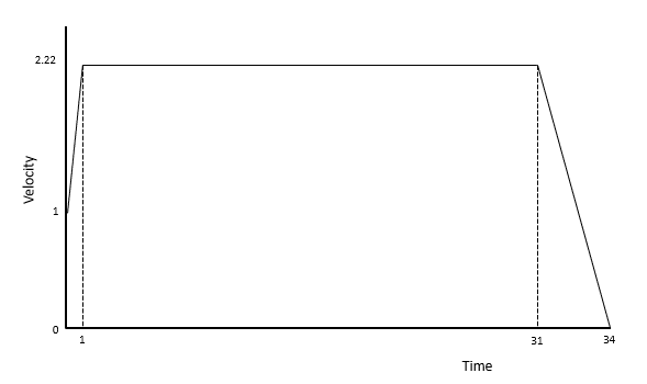
To find the distance, we can find the area of each section under the graph. It can be split into a trapezium, a rectangle and a triangle, so we have
\left( \dfrac{1}{2} \times (1 + 2.22) \times 1\right) + (30 \times 2.22) + \left( \dfrac{1}{2} \times 3 \times 2.22\right)
= 71.54\text{m}
Question 2: A train journey from Harrogate to London takes 4\text{ hours}. At t = 20\text{ minutes}, the train stops at Leeds for 10\text{ minutes}, before stopping at Sheffield, Nottingham and Leicester for \text{two minutes} each.
a) For which portion of the journey does the train move fastest?
b) When is it slowest (when not at a station)?
[2 marks]
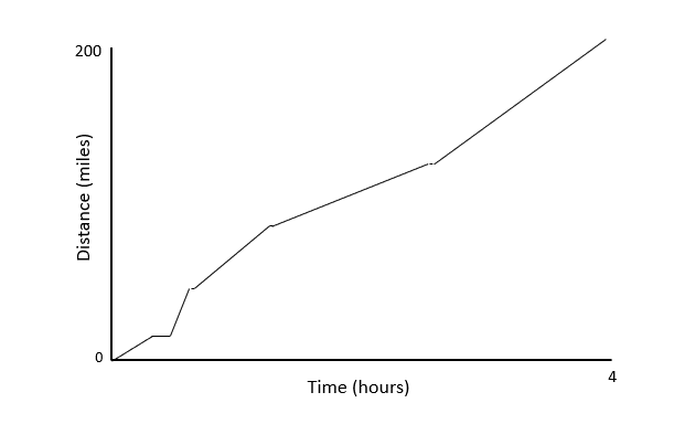
a) By inspection, we see that the graph is steepest (therefore travelling fastest) between the first and second stop, Leeds to Sheffield.
b) The graph is flattest (therefore travelling slowest) between the fourth and fifth stop, Nottingham to Leicester.
Question 3: A cyclist is travelling at 15\text{ ms}^{-1} and accelerates at a constant rate to 25\text{ms}^{-1}.
Using the graph, calculate her acceleration, and the distance travelled in that time.
[2 marks]
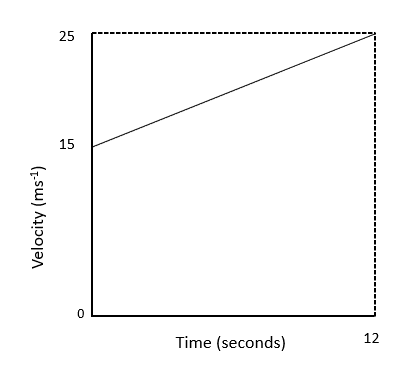
The change in velocity is 10\text{ ms}^{-1} over 12\text{ seconds}.
This indicates an acceleration of \dfrac{5}{6}\text{ ms}^{-2} = 0.833\text{ ms}^{-2}.
Using s = \dfrac{1}{2}(u + v)t, we have s = \dfrac{1}{2} \times 40 \times 12 = 240\text{ m}.
Motion Graphs Worksheet and Example Questions
SI Units
A LevelYou May Also Like...

MME Learning Portal
Online exams, practice questions and revision videos for every GCSE level 9-1 topic! No fees, no trial period, just totally free access to the UK’s best GCSE maths revision platform.
