Reduction to Linear Form
Reduction to Linear Form Revision
Reduction to Linear Form
Some exponential equations can be reduced to a form that looks like y=mx+c. Specifically, after applying the laws of logarithms we can treat y=ax^{n} and y=ab^{x} as if they were linear equations.
\mathbf{y=ax^{n}}
y=ax^{n}Take logarithms:
\begin{aligned}\log(y)&=\log(ax^{n})\\[1.2em]&=\log(a)+\log(x^{n})\\[1.2em]&=\log(a)+n\log(x)\end{aligned}
Overall we have:
y=ax^{n}\Rightarrow \log(y)=\log(a)+n\log(x)
Now if we plot \log(y) against \log(x), we have a straight line graph.
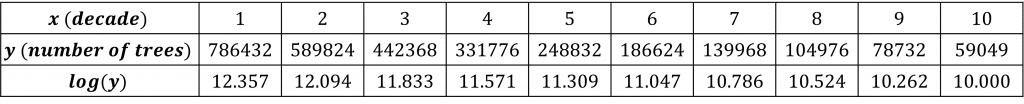
The graph below shows y against x in red and \log(y) against \log(x) in blue. As expected, the blue line is straight.

\mathbf{y=ab^{x}}
y=ab^{x}Take logarithms:
\begin{aligned}\log(y)&=\log(ab^{x})\\[1.2em]&=\log(a)+\log(b^{x})\\[1.2em]&=\log(a)+x\log(b)\end{aligned}
Overall we have:
y=ab^{x}\Rightarrow \log(y)=\log(a)+x\log(b)
Now if we plot \log(y) against x, we have a straight line graph.
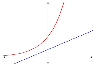
The graph below shows y against x in red and \log(y) against x in blue. As expected, the blue line is straight.


A Level Maths Predicted Papers 2024
The MME A level maths predicted papers are an excellent way to practise, using authentic exam style questions that are unique to our papers. Our examiners have studied A level maths past papers to develop predicted A level maths exam questions in an authentic exam format. The profit from every pack is reinvested into making free content on MME, which benefits millions of learners across the country.

A Level Maths Revision Cards
The best A level maths revision cards for AQA, Edexcel, OCR, MEI and WJEC. MME is here to help you prepare effectively for your A Level maths exams. The profit from every pack is reinvested into making free content on MME, which benefits millions of learners across the country.


Example 1: Converting to Linear Form
Convert y=99\times0.5^{x} to linear form.
[2 marks]
y=99\times0.5^{x}
\begin{aligned}\log(y)&=\log(99\times0.5^{x})\\[1.2em]&=\log(99)+log(0.5^{x})\\[1.2em]&=\log(99)+x\log(0.5)\end{aligned}
Example 2: Using Linear Form
The data below is taken from a plot of the form y=ax^{n}. By plotting \log_{10}(y) against \log_{10}(x), find a and n.
[5 marks]
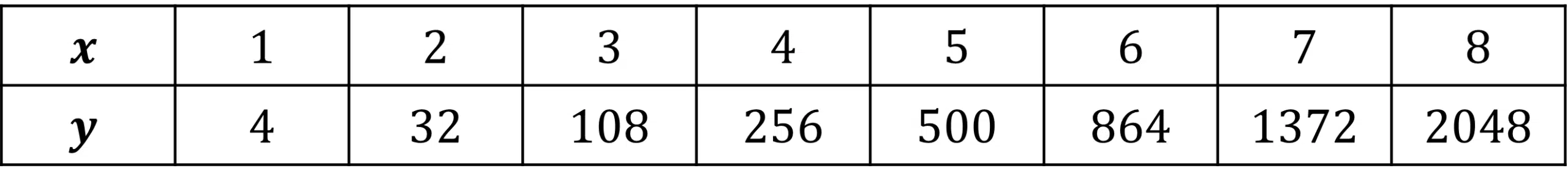
Step 1: Calculate \log_{10}(x) and \log_{10}y and put them in a table.

Step 2: Plot \log(y) against \log(x) on a scatter graph.

Step 3: Use the scatter graph to find the gradient and y-intercept.
Gradient is approximately \dfrac{3.3-0.6}{0.9-0}=\dfrac{2.7}{0.9}=3
y-intercept is approximately 0.6
Step 4: Use our linear form to interpret the gradient and y-intercept.
y=ax^{n}\rightarrow \log(y)=\log(a)+n\log(x)Gradient is n so n=3
y-intercept is \log(a) so \log(a)=0.6 so a=10^{0.6}=4 to two significant figures.
Step 5: Put together to determine the form of the plot:
y=4x^{3}
Reduction to Linear Form Example Questions
Question 1: The number of branches of a high-street store decreases over time. This trend, which is of the form y=ab^{x} is monitored over a number of years. Use the data from the monitoring to find a and b.
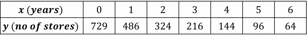
[5 marks]
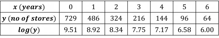
If the question does not specify a base for logarithms it is up to us to choose a sensible base. The choice of base should not affect the answer at the end. In the working below, we have used a base of 2.
Note the linear form:
y=ab^{x}\rightarrow log(y)=x\log(b)+\log(a)So the straight line is obtained by plotting \log(y) against x.
This means that we need to add a \log(y) row to the table.
Plot \log(y) against x and add a line of best fit.
Find the gradient and the y-intercept.
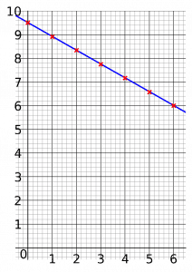
Gradient is \dfrac{6-9.5}{6-0}=\dfrac{3.5}{6}=-\dfrac{7}{12}
y-intercept is 9.5
Interpret the gradient and y-intercept.
Gradient is \log(b)
\log(b)=-\dfrac{7}{12}
b=0.667
y-intercept is \log(a)
\log(a)=9.5
a=729
Put it all together:
Our estimate for the line is y=729\times0.667^{x}
Question 2: The value of an investment in MathCoin is believed to reliably climb following an ax^{n} trajectory. Claire buys one MathCoin and monitors the price of her investment every month over one year. Find a and n.

[5 marks]
If the question does not specify a base for logarithms it is up to us to choose a sensible base. The choice of base should not affect the answer at the end. In the working below, we have used a base of 10.
Note the linear form:
y=ax^{n}\rightarrow log(y)=n\log(x)+\log(a)So the straight line is obtained by plotting \log(y) against \log(x).
This means that we need to add a \log(x) row and a \log(y) row to the table.
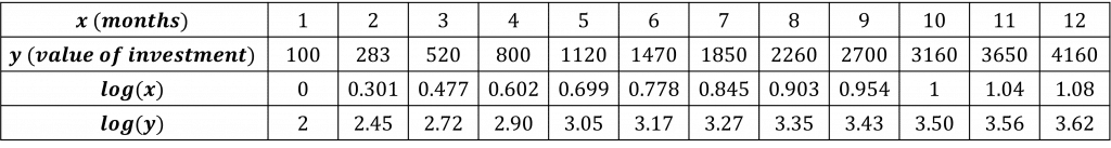
Plot \log(y) against \log(x) and add a line of best fit.
Find the gradient and the y-intercept.
Gradient is \dfrac{3.5-2}{1-0}=\dfrac{1.5}{1}=1.5
y-intercept is 2
Interpret the gradient and y-intercept.
Gradient is n
n=1.5
y-intercept is \log(a)
log(a)=2
a=100
Put it all together:
Our estimate for the line is y=100\times x^{1.5}
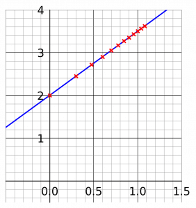
Question 3: A forest has been declining in population since the nineteenth century. To assess this decline, a census of the tree population of the forest was conducted every ten years in the twentieth century. It is believed this decline follows a y=ab^{x} curve. Use the table of census data to find a and b.

[5 marks]
Again we can choose our own base for logarithms, so we will take the logarithm with base 3.
y=ab^{x}
\begin{aligned}\log(y)&=\log(ab^{x})\\[1.2em]&=\log(a)+\log(b^{x})\\[1.2em]&=\log(a)+x\log(b)\end{aligned}
So we plot \log(y) against x, and the gradient will be \log(b) and the y intercept will be \log(a).
Plotting \log(y) against x gives this graph.
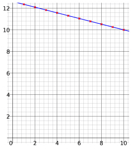
The graph goes through the points (1,12.357) and (10,10).
\begin{aligned}\text{gradient}&=\dfrac{10-12.357}{10-1}\\[1.2em]&=\dfrac{-2.357}{9}\\[1.2em]&=-0.262\end{aligned}
\log(b)=-0.262
b=3^{-0.262}
b=0.750
The graph passes through (1,12.357) and has a gradient of -0.262, so it also passes through (0,12.357+0.262)=(0,12.619)
So y intercept is 12.619
\log(a)=12.619
a=3^{12.619}
a=1048576
Hence, y=1048576\times0.750^{x}
You May Also Like...

MME Learning Portal
Online exams, practice questions and revision videos for every GCSE level 9-1 topic! No fees, no trial period, just totally free access to the UK’s best GCSE maths revision platform.
